Grass Interaction - Part 1

Grass Interaction, a staple in any game that has grass, and an inevitable when making open-world games (unless you are making a scorched land). However, most of the tutorials out there seem to be a little limited when it comes to make natural-looking grass interaction. Most would stop at the trample effect - which is ok for basic use cases. The problem becomes more complex when you add NPCs or making a bouncing effect.

To fill the gap, this series aim to provide a slightly overkill simulation of grass interaction - by overkill I mean it won’t be frame-rate friendly since we will be doing lots of expensive calculations. You could simplify the calculations depending on your project need.

Overview#

We will achieve the following effects:

Grass is trampled when very near an instigator.
Grass curves outwards when near an instigator.
Grass will gradually restore its position after leaving the influence of an instigator.
Grass may show some oscillation during the restoration process.
Each grass can have its own elasticity constant and damping coefficient.
Support multiple instigators.

grass oscillation

We will improve grass interaction based on the most basic method - adding a displacement in the vertex shader. There are plenty of other methods that provide better simulations, for example, using bone animation, suitable for more detailed plants. The technique we are using assumes the following conditions:

Newtonian physics applies - we only deal with macro, low-velocity objects.
Grass width is significantly smaller than instigators - like grass vs human in real life. If your game is about grass vs cricket, then this technique is suboptimal.
No precise physical simulation needed - we will make lots of simplifications and compromises to achieve a visually correct result, but these simplifications will make the simulation not strictly physically correct.

The series is divided into 5 parts:

Part 1 (this post): physical abstraction of grass, instigators, and relevant theories.
Part 2: Calculating influence of instigators.
Part 3: Send influence data to the GPU.
Part 4: Applying vertex displacement.
Part 5: Adjustments and Refinements.

NOTE: The theoretical part requires you to have some college level calculus and Newtonian physics knowledge to understand completely. In fact, it would be very similar to a first year physics course. But it is OK if you don’t understand everything - it is not required to achieve the effects mentioned above.

Now let’s dive into the theory.

Physical Abstraction of Grass#

Formulation of the System#

We want to reduce the grass interaction problem to a well-studied physical system. What could it be, then?

Empirically, the movement of grass resembles a mass attached to an elastic rod. One end of the elastic rod is attached to the ground and is immobile, the other end is attached to the mass. The elastic rod can be bent but cannot be compressed. For simplicity, the mass of the elastic rod is ignored.

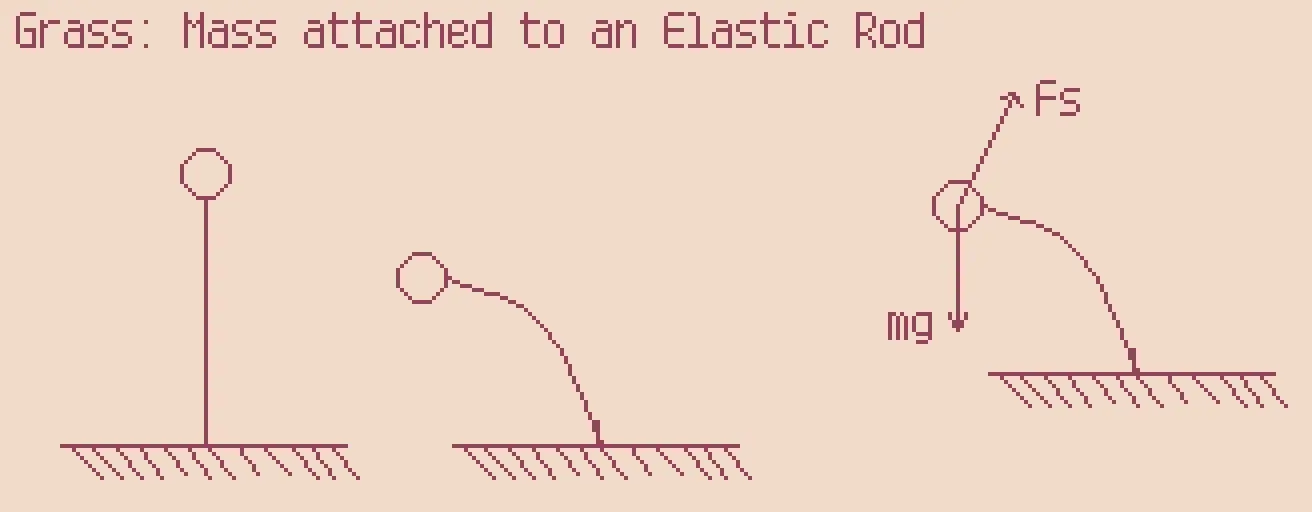
Though this simplification is still too complex for us, due to the rod being bendable and changing the straight distance between the mass and the root. What we can do is to assume the rod is non-bendable (rigid), but still providing elastic force $F_s$ . Imagine there is a hidden contraption at the root of the grass, driven by a spring, whenever the grass isn’t upright, the contraption provides the elastic force to restore the upright position.

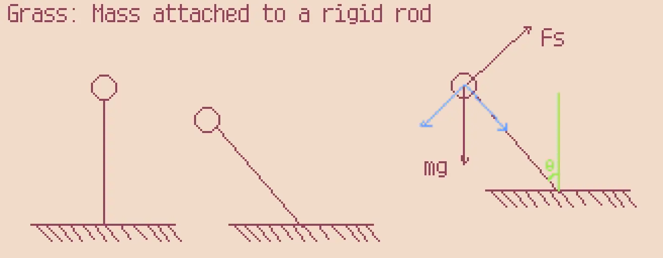
If you now flip your monitor upside down, you might recognize this diagram in other literature: This is very similar to a damped/driven pendulum system, except it is upside down, and that is indeed a well-studied physical system.

Force Analysis#

Our goal is to obtain an analytical expression $\theta(t)$ that, given elapsed time $t$ , we obtain the signed angle $\theta$ .

Assume the signed angle between the up direction and the rigid rod is $\theta$ :

$Fs$ is the elastic force perpendicular to the rigid rod and always pointing towards the upright position. Similar to Hooke’s Law, this force is proportional to angle $\theta$ . Hence, $Fs=m*k*\theta$ where $k$ is the elasticity of the grass.
The gravity $G$ can be decomposed into a force that goes along the rigid rod $Gy$ and another that is perpendicular to the rigid rod, in the opposite direction of the elastic force $Gx$ . $Gy$ is balanced out by the supportive force of the rigid rod, then it only leaves $Gx$ our point of interest. With a little trigonometry, we can find $Gx = sin(\theta)*m*g$
Another damping force $D$ proportional to the angular velocity of the mass: $D = \frac{d\theta}{dt}*b*m$ where $b$ is the damping coefficient. This force opposes the direction of the velocity.

NOTE: Usually we do not multiply damping force by mass. But since both $b$ and $m$ are invariant during the simulation, $b*m$ can be seen as just a constant of the grass that replaces the conventional damping coefficient.

Therefore, with the 2nd law:

a = \frac{d^2x}{dt^2}=k*\theta- sin(\theta)*g - \frac{d\theta}{dt}*b

We know that linear displacement can be expressed as $dx = l_0*d\theta$ where $l_0$ is the length of the rod. Derive the expression 2 times, then we will have:

\frac{d^2x}{dt^2} = l_0*\frac{d^2\theta}{dt^2} = k*\theta- sin(\theta)*g - \frac{d\theta}{dt}*b

Simplify the equation and we have a familiar form:

l_0*\frac{d^2\theta}{dt^2} + b*\frac{d\theta}{dt} + g*sin(\theta) - k*\theta = 0

This equation is nonlinear because of the $g*sin(\theta)$ term, and we have to do a classic trick to make it solvable analytically - Small Angle Approximation.

The following graph shows $f(x) = sin(x)$ (green), $f(x) = x$ (red) and $f(x)=x-\frac{x^3}{6}$ (blue).

Around 28 degrees (0.5 radians), we can see that $f(x) = x$ is very close to $f(x) = sin(x)$ . The Taylor expansion with 2 terms $f(x)=x-\frac{x^3}{6}$ gives a better approximation, but it doesn’t make the equation easier to solve.

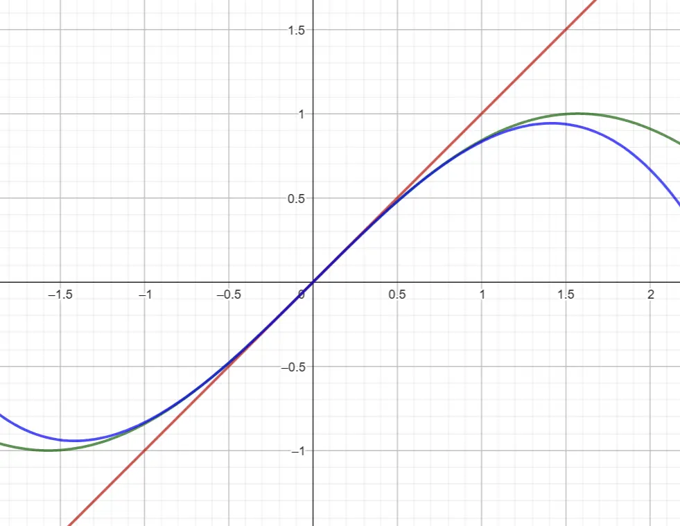
However, remember that we do not need a strictly physical simulation, we just need it to be visually correct. So we will use $x$ to approximate $sin(x)$ in all cases. Our equation now becomes:

\frac{d^2\theta}{dt^2} + \frac{b}{l_0}*\frac{d\theta}{dt} + \frac{g-k}{l_0}*\theta = 0

We now assume:

$\gamma=\frac{b}{2*l_0}$
$\omega_0 = \sqrt{\frac{g-k}{l_0}}$

then we can simplify the equation to an even more familiar form:

\frac{d^2\theta}{dt^2} + 2\gamma*\frac{d\theta}{dt} + \omega_0^2*\theta = 0

Solving the Differential Equation#

We will now use the Exponential Guess method:

Guess an exponential solution of the form $Ae^{\alpha t}$
Derive the condition $\alpha$ must satisfy in order for $Ae^{\alpha t}$ to be a solution of the equation.
Solve the condition for values of $α_1,...,α_n$
If the $α_i$ are unique, write general solution as $x(t) = A_1e^{\alpha_1 t}+A_2e^{\alpha_2t} + ··· + A_ne^{\alpha_nt}$ .

If $\theta(t)$ is of form $Ae^{\alpha t}$ then:

A(\alpha^2+2\gamma\alpha+\omega_0^2)e^{\alpha t}=0

Which means:

\alpha^2+2\gamma\alpha+\omega_0^2=0

And the solution for $\alpha$ is

\alpha = -2\gamma \pm \sqrt{\gamma^2-\omega_0^2}

Depending on the value of $\gamma$ and $\omega_0$ , we can have 3 different cases:

$\omega_0>\gamma$ : weak damping or underdamped
$\omega_0=\gamma$ : critical damping or critically damped
$\omega_0<\gamma$ : strong damping or overdamped

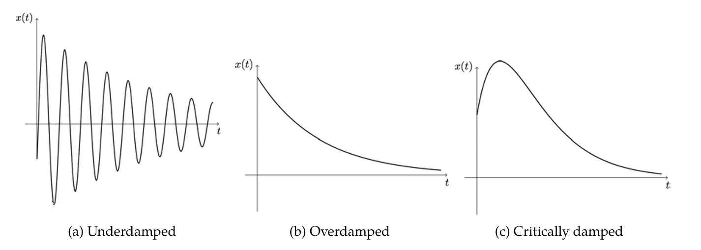
we also note:

\omega = \sqrt{abs(\gamma^2-\omega_0^2)}

Now to properly solve the equations we need some initial conditions. In our grass simulation, we assume the grass has no initial velocity when it leaves an instigator’s influence, and we can write the initial conditions as follows:

$\theta(0)=\theta_0$ (initial angle)
$\frac{d\theta(0)}{dt}=0$ (no initial velocity)

Underdamped#

When underdamped, the solution to our equation is complex:

\theta(t)=A_1e^{\alpha_1 t}+A_2e^{\alpha_2 t} = e^{-\gamma t}(A_1e^{i\omega t}+A_2e^{-i\omega t})

But since we need a real solution, we can just take the real part (recall Euler’s formula $e^{it}=cos(t)+isin(t)$ ):

\theta(t)=e^{-\gamma t}(A_1cos(\omega t)+A_2sin(\omega t))

since cos and sin are only different in phase, we can further rewrite the previous solution as

\theta(t)=A_0*e^{-\gamma t}cos(\omega t-\phi)

We only need to use initial conditions to solve $A_0$ and $\phi$ now.

given $\frac{d\theta(0)}{dt}=0$ we have $\phi = 0$
given $\theta(0)=\theta_0$ we have $A_0 = \theta_0$

Hence, for underdamped case, we have

\theta(t)=\theta_0*e^{-\gamma t}cos(\omega t)

Overdamped#

Similar to underdamped, but without the imaginary:

\theta(t)=A_1e^{\alpha_1 t}+A_2e^{\alpha_2 t} = e^{-\gamma t}(A_1e^{\omega t}+A_2e^{-\omega t})

with the initial conditions:

given $\theta(0)=\theta_0$ we have $A_1+A_2 = \theta_0$
given $\frac{d\theta(0)}{dt}=0$ we have $A_1-A_2=\frac{\gamma\theta_0}{\omega}$

Solve them and we get

A_1 = \frac{\theta_0}{2} + \frac{\gamma\theta_0}{2\omega}

and

A_2 = \frac{\theta_0}{2} - \frac{\gamma\theta_0}{2\omega}

Critically Damped#

In this case we have non-unique solution for $\alpha$ and we must write the solution in another form (note that we have $\omega_0 = \gamma$ then $\alpha = -\gamma$ ):

\theta(t) = (A+Bt)e^{-\gamma t}

Again, applying our initial conditions:

given $\theta(0)=\theta_0$ we have $A = \theta_0$
given $\frac{d\theta(0)}{dt}=0$ we have $B=\gamma\theta_0$

Hence,

\theta(t) = \theta_0(1+\gamma t)e^{-\gamma t}

Now we have everything we need to describe the movement of the grass when the instigator’s influence disappears!

Physical Abstraction of Instigators#

Now the problem is how we determine the initial condition $\theta_0$ mentioned above. And this initial angle is tied to the shape of the instigator.

We assume the height of the instigator can be defined as a function $h(x)$ where $x$ represents the distance between the center of the instigator and the root of the grass.

A simple approach would be to use linear interpolation:

h(x) = cx

where c is an instigator-specific constant.

Second Order Polynomial#

In our case, let us do something a little bit more unnecessary: use a curve instead.

h(x) = cx^2=\frac{h_0}{R_0^2}x^2

NOTE: Later, I found out that I overlooked a crucial aspect - $\theta(R_0) = 0$ . This is not easily satisfied when using a second order polynomial with the tangent case simplification. Eventually I would end up using elliptic curve as it guarantees $\frac{dh(R_0)}{d(d)}=tan(\pi/2)$ . But I still leave the polynomial reasoning here to demonstrate the thought process. If you don’t care about it, jump to the ellipse section.

Where:

$h_0$ is the height of the instigator.
$R_0$ is the radius of the instigator.

The advantage of using a second order function is that it resembles placing a capsule collider which is exactly what a character controller looks like.

Grass has a fixed length of $l_0$ , thus we can use a segment $g(x)=p(x-d)$ to express it, where $d$ is the distance between the center of the instigator and the root of the grass. It also means we may have 2 cases to deal with when trying to solve the initial angle:

Tangent Case: the grass blade is a tangent of the instigator curve.
Non-tangent Case: the grass blade’s extremity touches the instigator curve.

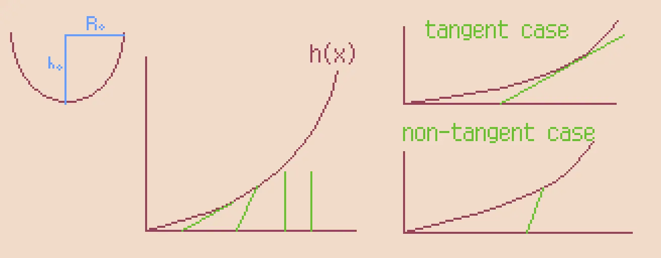
Tangent Case#

Assume the intersection between the grass segment and the curve is $x_0$ . The derivative of the curve at $x_0$ provides the slope of the grass segment. Hence:

$p=h'(x_0)=2cx_0$

And since the line intersects with the curve at $x_0$ , we have:

$x_0^2*c=2cx_0(x_0-d)$

after simplification:

$x_0 = 2d$

the grass equation becomes:

$g(x)=4cd(x-d)$

and we have:

$\theta_0(d) = \frac{\pi}{2}-arctan(4cd)$

Non-tangent Case#

In this case, the intersection is $(x_0,cx_0^2)$ by evaluating the instigator curve at $x_0$ . The displacement relative to $(d,0)$ is $(x_0-d,cx_0^2)$ . This vector has length of $l_0$ . Then:

$(x_0-d)^2+c^2*x_0^4=l_0^2$

after expansion:

$c^2*x_0^4+x_0^2-2d*x_0+(d^2-l_0^2)=0$

Unfortunately, this is not practical to solve. But remember we are not doing physically accurate simulation, so we will treat the non-tangent case as tangent case.

The issue#

The polynomial approach has a major issue that I only discovered later - it can create discontinuity at $R_0$ where we expect 0 degrees:

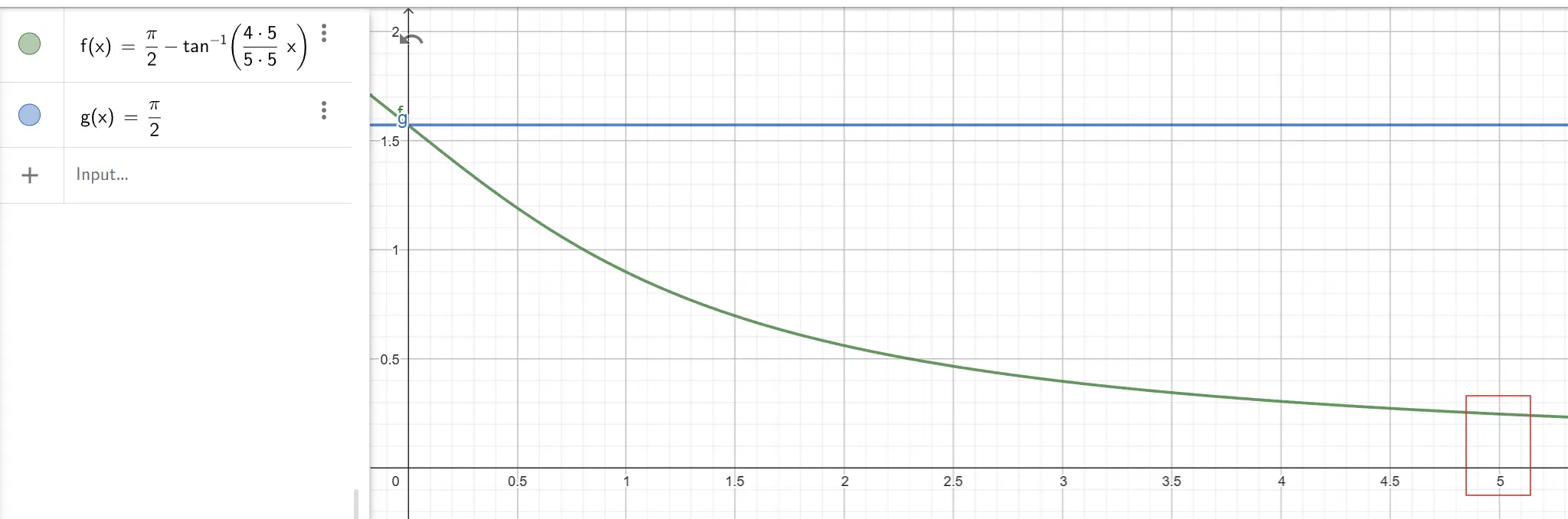
This is a fairly noticeable discontinuity and causes grass blade to sort of “teleport” when entering an entity’s influence.

Here’s a better illustration of the problem:

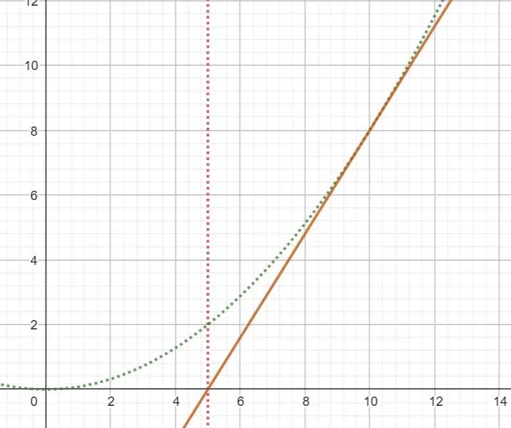
The curve has $h_0 = 2$ and $R_0 = 5$ , ideally; we wish the grass whose root is at 5 to be close to upright, because anything outside of 5 should be upright. However, in the above diagram, we can see that the tangent of the curve passing point (5,0) is not at all upright. This means any grass that touches the rim of the object will suddenly lean with that angle, resulting in visual jitters.

To eradicate this problem, we need to change how the object is abstracted, And the curve that has a slope of 0 at origin and a slope of infinity (perpendicular to the x axis) at $R_0$ , is part of an ellipse.

Ellipse#

We now model the instigator as an ellipse, and its equation would look like this:

$\frac{y^2}{h_0^2}+\frac{x^2}{R_0^2}=1$

NOTE: $y$ is $h(x)$ seen in the polynomial approach.

This ellipse doesn’t pass through $(0,0)$ and $(R_0,h_0)$ , but $(R_0,0)$ and $(0,-h_0)$ . For now, it is fine, because what we will calculate is the slope of the tangent, which doesn’t change even if we move the ellipse.

To obtain the slope $\frac{dy}{dx}$ , we derive by $\frac{d}{dx}$ :

$\frac{2}{h_0^2}*y*\frac{dy}{dx}+\frac{2}{R_0^2}*x = 0$

After simplification, we obtain:

$\frac{dy}{dx}=-\frac{h_0^2}{R_0^2}\frac{x}{y}$ Now we need to find a point $(x_0,y_0)$ on the ellipse to calculate the value of the slope.

We already know that the tangent should pass through $(d,0)$ , but since our ellipse is shifted down $h_0$ units, the point becomes $(d,-h_0)$ . The tangent equation of an ellipse is given by:

$\frac{x_0x}{R_0^2}+\frac{y_0y}{h_0^2} = 1$

Substitute with $(d,-h_0)$ , we obtain

$\frac{x_0d}{R_0^2}-\frac{y_0h_0}{h_0^2} = 1$ moving the terms around, we get

$y_0=h_0(\frac{x_0d}{R_0^2}-1)$ Now we plug it back to the ellipse equation:

$\frac{(h_0(\frac{x_0d}{R_0^2}-1))^2}{h_0^2}+\frac{x_0^2}{R_0^2}=1$

which simplifies to:

$x_0((R_0^2+d^2)x_0-2R_0^2h_0)=0$ we have 2 solutions, either $x_0=0$ (valid but not what we are interested in), and

$x_0=\frac{2R_0^2h_0}{R_0^2+d^2}$

then we plug it back to the $y_0$ equation we have

$y_0 = h_0(\frac{2d^2}{R_0^2+d^2}-1)$ with these we can express the slope as a function of $d$ :

$\frac{dy}{dx}=-\frac{h_0^2}{R_0^2}\frac{\frac{2R_0^2h_0}{R_0^2+d^2}}{h_0(\frac{2d^2}{R_0^2+d^2}-1)}=\frac{2h_0d}{R_0^2-d^2}$ Finally, we can express the initial angle as

$\theta_0(d) = \frac{\pi}{2}-arctan(\frac{2h_0d}{R_0^2-d^2})$

Here’s the initial angle curve for an instigator that has 10 radius and 3 height, we can see the curve approaches 0 when approaching 10 from the left:

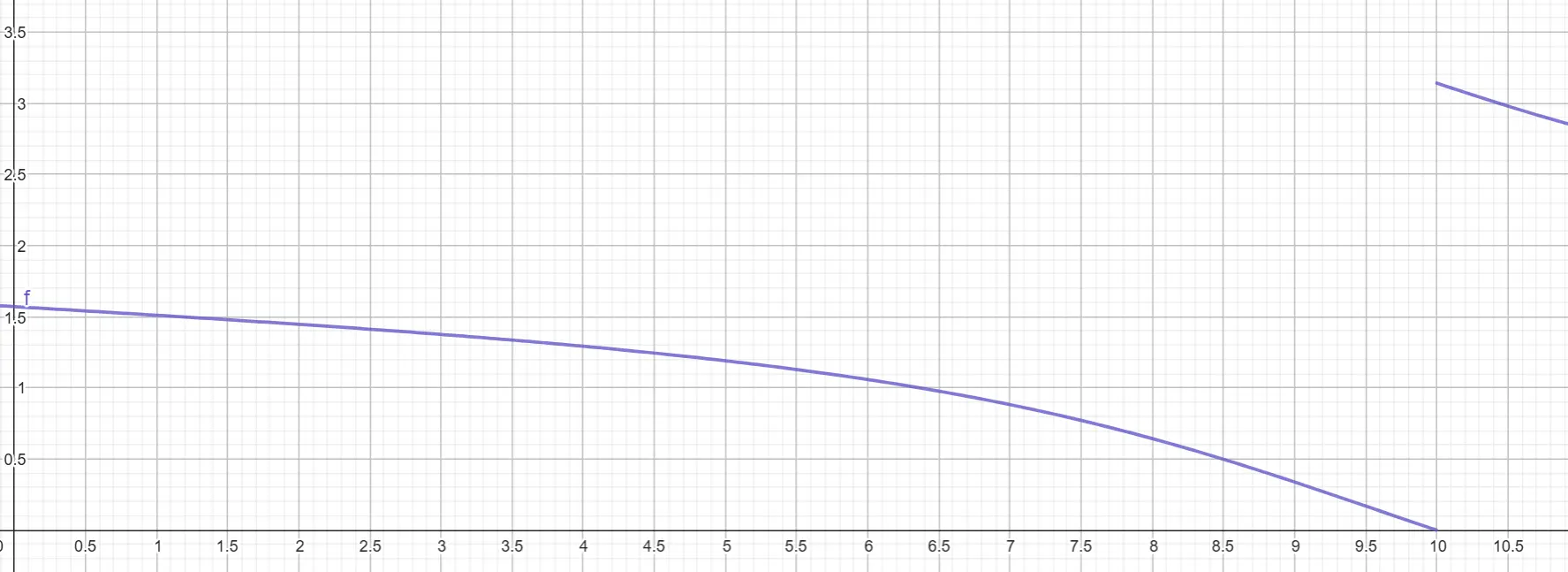
We must take precautions in this case : when $d=R_0$ , we have division by zero. and we must account for it in shader.

We will need to express $y$ with $x$ later, and this time we must move the ellipse up by $h_0$ units:

$\frac{(y-h_0)^2}{h_0^2}+\frac{x^2}{R_0^2}=1$

After simplification, we have

$y=h(x)=h_0(\sqrt{1-\frac{x^2}{R_0^2}}+1)$

Conclusion#

We established the 3 cases for grass motion $\theta(t)$ :

Underdamped : $\theta(t)=\theta_0*e^{-\gamma t}cos(\omega t)$
Overdamped: $\theta(t)= e^{-\gamma t}(A_1e^{\omega t}+A_2e^{-\omega t})$ where $A_1 = \frac{\theta_0}{2} + \frac{\gamma\theta_0}{2\omega}$ and $A_2 = \frac{\theta_0}{2} - \frac{\gamma\theta_0}{2\omega}$
Critically damped: $\theta(t) = \theta_0(1+\gamma t)e^{-\gamma t}$

With:

$\gamma=\frac{b}{2*l_0}$
$\omega_0 = \sqrt{\frac{g-k}{l_0}}$
$\omega = \sqrt{abs(\gamma^2-\omega_0^2)}$

And a way to express initial angle $\theta_0$ with an elliptic instigator:

$\theta_0(d) = \frac{\pi}{2}-arctan(\frac{2h_0d}{R_0^2-d^2})$

The height of the lower surface of the instigator at $d$ relative to its lowest point is expressed as

$h(d)=h_0(\sqrt{1-\frac{d^2}{R_0^2}}+1)$

In part 2 we will record the influence of the instigator (its position, velocity, and some calculated results) to fuel the eventual calculation in the vertex shader.